Biodiversity Heritage Library - Program news and collection highlights from BHL
  • Home
  • News
  • Featured Books
    • All Featured Books
    • Book of the Month Series
    • BHL at 20
  • User Stories
  • Campaigns
    • Fossil Stories
    • Garden Stories
    • Monsters Are Real
    • Page Frights
    • Her Natural History
    • Earth Optimism 2020
  • Tech Blog
  • Visit BHL
Home
News
Featured Books
    All Featured Books
    Book of the Month Series
    BHL at 20
User Stories
Campaigns
    Fossil Stories
    Garden Stories
    Monsters Are Real
    Page Frights
    Her Natural History
    Earth Optimism 2020
Tech Blog
Visit BHL
  • Home
  • News
  • Featured Books
    • All Featured Books
    • Book of the Month Series
    • BHL at 20
  • User Stories
  • Campaigns
    • Fossil Stories
    • Garden Stories
    • Monsters Are Real
    • Page Frights
    • Her Natural History
    • Earth Optimism 2020
  • Tech Blog
  • Visit BHL
Biodiversity Heritage Library - Program news and collection highlights from BHL
Blog Reel, Tech Updates

OCR Improvements: An Early Analysis

Color coded comparison of OCR text highlighting the differences in text recognition

Optical character recognition (OCR) plays a critical part in BHL’s contributions to the scientific community. OCR in and of itself is a remarkable achievement, converting images of typewritten text to computer-readable text with “pretty good” accuracy. OCR on handwritten text is an even greater challenge to address and is beyond the scope of the improvements discussed here. The scientific work that BHL supports demands the best accuracy that we can provide using available tools, and let’s be honest, available budgets.

Recently, our colleagues at the Internet Archive made the transition away from the ABBYY FineReader OCR software to the Tesseract Open Source OCR engine. Over the past year or more, the OCR team at the Internet Archive has adapted and fine-tuned Tesseract to their workflows. Our first impression is that Tesseract OCR is more than “pretty good” in its ability to identify text from the page images provided to it.

The downside to this is that the Internet Archive has rightfully chosen to not re-process all existing text content through the Tesseract OCR engine. This is a prohibitively expensive and time-consuming prospect given that they have 35 million text-based items and reprocessing them would take several years and use up resources that could otherwise be used for gathering new content.

However, in the interests of supporting the efforts of the BHL community, the BHL Tech Team is working with our Internet Archive partner to reprocess some of BHL’s oldest content with the newest available version of Tesseract OCR. We are currently in a testing phase, and this blog post details some of our early results.

Selection

The first step in the process was to identify which versions of which OCR engine was used on BHL’s content. This was a simple matter of checking the “OCR” metadata value at the Internet Archive for each of the 263,000 items at BHL. The results as of December 2020 were:

“OCR” Metadata Value Count
ABBYY FineReader 8.0 80,447
ABBYY FineReader 9.0 35,276
ABBYY FineReader 11.0 45,679
ABBYY FineReader 11.0 (Extended OCR) 49,086
Tesseract 4.1.1 83
No OCR value  39,530

We suspect that those items with No OCR value are the very oldest content at BHL and were processed with an unknown OCR engine, or ABBYY FineReader 8.0 or earlier.

For a test and ultimately for moving forward with reprocessing, we chose the 80,000 items with ABBYY FineReader 8.0. We will likely add the other 39,500 items with No OCR value.

The Process

The steps to reprocess the OCR for an item are simple. We delete a few critical files at the Internet Archive and issue a “derive” command to restore them. In doing so, the OCR is regenerated and the “OCR” metadata value is updated accordingly.

The challenging part of the process is time and resources. OCR is a computationally expensive process and it can take dozens of minutes to several hours to create the OCR for a single Item. We also must be aware that we can potentially take computing resources from other activities at the Internet Archive, so we issue the “derive” command at a lower priority than other Internet Archive activities, effectively using up spare or unused resources as they are available.

In other words, we’re being good citizens of the Internet Archive ecosystem.

The Results

Since this is what you came for, in summary, the results are very good and this is a worthwhile effort.

Our tests for evaluating the results are a combination of visual inspection and computational analysis. For backup and local analysis purposes, BHL keeps a copy of all content at the Internet Archive, but its updates are currently disabled during this testing phase. Using this backup copy as the source of “old” content, we can compare it to the “new” content at the Internet Archive.

Analysis 1: Misspellings

The first analysis is to simply check for misspelled words. While at first glance this seems too simplistic, OCR operates on a letter-by-letter analysis of the text and often has challenges correctly identifying a letter and will often produce invalid words.

Using the Linux aspell tool, we can find misspelled words and count them using a command such as the following:

cat FILENAME | aspell list | wc -l

This command sends the contents of FILENAME to aspell, which lists misspelled words, one per line, then sends that list to the word-count wc command to list the number of lines. Using a test case of 1955seventyoneye1955harr, we count the misspellings for the old and new versions:

  • Old OCR Text (from 2013): 2,357 misspelled words
  • New OCR Text (from 2020): 1,639 misspelled words

There are expected commonalities between the two lists of misspelled words. Proper or scientific names such as Elberta and Harrison or varietal names such as Dixired or Redhaven don’t exist in the standard English dictionary. Additionally, legitimate misspellings in the printed text appear, such as Recomemnded, appear in the results. Regardless, the greatly reduced number of misspellings is a good indicator of OCR accuracy. 

Analysis 2: Visual Inspection

One of the most important downstream effects of improved OCR is improved identification of scientific names. BHL partners with the Global Names Architecture (GNA) to identify scientific names in the BHL text. Focusing on this, we can see that improvements in the OCR reveal more scientific names that were missed in the past.

Example A: Ligustrum ovalifolium

The original page image at BHL discusses the California Privet (Ligustrum ovalifolium).

The OCR comparison of the old engine (in red) and the new (in green) shows that the new Tesseract OCR engine was better able to convert the words to text. This will ultimately cause this name to appear in BHL’s list of scientific names on this page of the document where currently it may not appear.
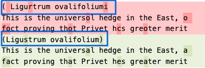
Color coded comparison of OCR text highlighting the differences in text recognition

Example B: Multiple names

A second example showing numerous taxon names that are now correctly identified by the OCR. It’s worth mentioning that this page in BHL includes the genus (Magnolia or Lonicera) but not the full species name. We expect that the full name will appear in BHL with the improved OCR.
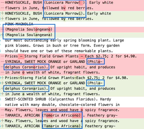
Color coded comparison of OCR text highlighting differences in text recognition

Analysis 3: Scientific Name Finding

As mentioned earlier, BHL partners with the Global Names Architecture (GNA) to identify scientific names in the OCR content of BHL. While we use APIs to perform this function, GNA also offers a command line tool to process a body of text to identify scientific names.

Similar to counting the misspelled words, we use a series of Linux commands to process the OCR text and count the scientific names found in the text.

gnfinder find FILENAME  -c -s 1,3,4,9,11,12,167,172,179,181 |
  jq '.names[] .verification.BestResult.matchedName' | 
  sort | uniq | wc -l

gnfinder is the command to find the scientific names. This command returns JSON content, which we then send to the jq command to count the number of BestResult.matchedName elements in the JSON. Then we sort, get the unique names, and count them with wc. A sample of the JSON output looks like:

{
  "type": "Uninomial",
  "verbatim": "(Lonicera",
  "name": "Lonicera",
  "odds": 93678.22872366496,
  "annotation": "",
  "verification": {
    "BestResult": {
      "dataSourceId": 1,
      "dataSourceTitle": "Catalogue of Life",
      "taxonId": "4091239",
      "matchedName": "Lonicera",
      "matchedCanonical": "Lonicera",
      "currentName": "Lonicera",
      "classificationPath": 
        "Plantae|Tracheophyta|Magnoliopsida|Dipsacales|
           Caprifoliaceae|Lonicera",
      "classificationRank": 
        "kingdom|phylum|class|order|family|genus",
      "classificationIDs": 
        "3939764|3942634|3942724|3942969|3942971|4091239",
      "matchType": "ExactMatch"
    }
  },
  [...]
}

Counting these for our example 1955seventyoneye1955harr, we find:

  • Old OCR Scientific Names: 20 unique names found
  • New OCR Scientific Names: 38 unique names found

This is a simple case indicating that an additional 18 unique names were found in the content. Taking a random sample of 10 other items shows the following larger differences in the number of unique scientific names found:

Item Identifier Unique Names Found in OCR
Old New
guidebooksofexcu03inte 190 190
dissectionofdoga00howe 23 25
ueberliasbeta00schl 38 55
mobot31753003413330 641 920
CUbiodiversity1249031-9750 1,042 1,244
annalesdelasoci2627188283soci 2,786 3,046
weiterebeobachtu00kl 59 62
verhandlungender42zool 2,487 2,806
etudedesfleu1865cari 1,077 1,148
bulletinbiologiq47univ 750 1,127

It is worth noting that a visual inspection of these names indicates there is some fine-tuning remaining. gnfinder identifies both binomial names (genus and species) and uninomial names (genus only) in the content. There look to be instances where names are found in the new OCR that don’t exist in the content, but are incorrectly being identified as uninomials. gnfinder provides a type of score that must be fine tuned for the new OCR in order to reduce this effect. This is a task for future discussion.

Summary

While there is further work to do in loading this new content into BHL and in the scientific-name-finding part of the process, these initial results are encouraging and are enough to help us make the decision to continue reprocessing the OCR using the Internet Archive’s installation of Tesseract OCR.

This journey is years in length. Even if we were to process at the highest priority (something we would never consider), we are planning to affect nearly half of BHL’s 263,000 items. Our current rate of progress at the aforementioned lower priority is approximately 100 items per day. At such a pace, the 120,000 items will take three years to complete.

Future blog posts will occur as there are more updates to share with the BHL community.
July 19, 2022by Sheila Rabun
Blog Reel, User Stories

What’s This Bird? Classify Old Natural History Drawings with R

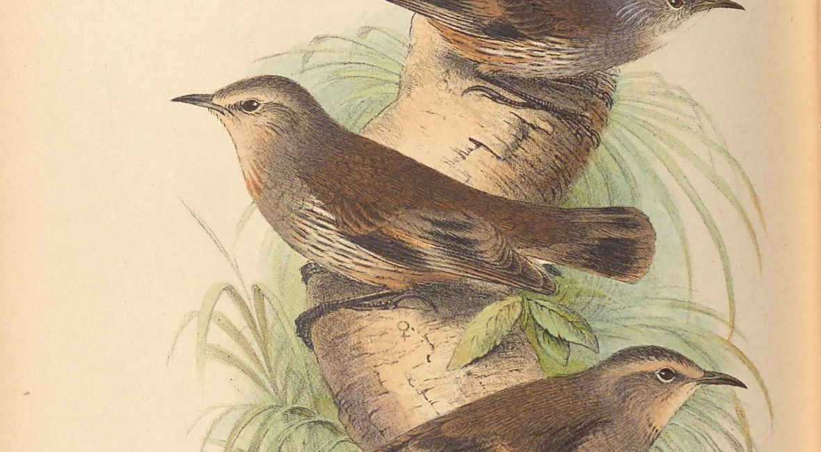
illustration of birds

This post was originally published on the rOpenSci blog on 28 August 2018 and is republished with permission of the author, Dr. Maëlle Salmon, and rOpenSci.

Armed with rOpenSci’s packages binding powerful C++ libraries and open taxonomy data, how much information can we automatically extract from images? Maybe not much, but, experimenting with gorgeous drawings from a natural history collection, we can least explore image manipulation, optical character recognition (OCR), language detection, and taxonomic name resolution with rOpenSci’s packages.

Free natural history images and appropriate R tooling!

A long time ago I had bookmarked the Flickr account of the Biodiversity Heritage Library (BHL). So many beautiful images of biodiversity, moreover free to use! In particular, I downloaded all pictures from one of the Birds of Australia albums (contributed in BHL by Museums Victoria).

I wanted to try to extract the bird names from images using packages of Jeroen Ooms’, rOpenSci’s post-doc hacker & C(++)-bindings wizard. For that I worked with magick for image manipulation, tesseract for optical character recognition (OCR), cld2/cld3 for language detection… Quite the armory! We’ll also sprinkle some taxonomy magic by Scott Chamberlain, one of rOpenSci’s co-founders, to resolve the names extracted.

OCR bird naming workflow, piece by piece

In this section, we explain the different elements of our R workflow: preparing images, extracting text, resolving taxonomic names.

Image preparation

I saved the pictures locally in a “birds” folder. Yes, I click-buttoned instead of using the Flickr API for which e.g. Jim Hester wrote a minimal R wrapper… I don’t do everything with R scripts (yet).

library("magrittr") 
filenames <- fs::dir_ls("birds")

Each image shows a bird and its name. Images are either landscape- or portrait-oriented, but for the sake of simplicity, I’ll act as if they were all portrait-oriented. A possible easy and lazy fix here would be to duplicate images rotated (magick::image_rotate) in all possible directions and then to apply the workflow to all 4 versions of each image, hoping to get good data from one of the rotated versions.

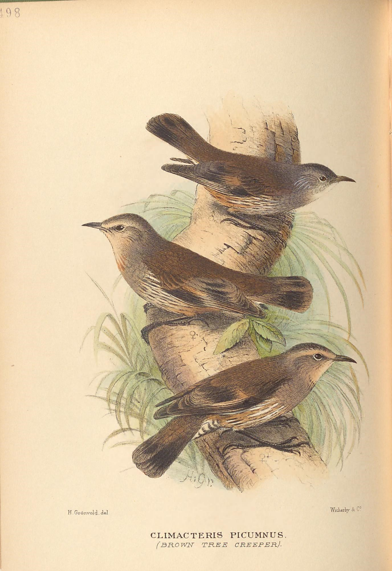
magick::image_read(filenames[1])
illustration of birds

Mathews, Gregory M. The Birds of Australia. v. 11 (1923-24). Art by Henrik Grönvold. Contributed in BHL from Museums Victoria.

From that image, I wanted to extract the name indicated below the bird. To maximize the efficiency of OCR, I shall first prepare the image, since the accuracy of OCR depends on the quality of the input image which can be influenced a bit. This part could be tweaked even more, and in real life examples it’ll be worth spending time trying different magick functions and parameter values. Since I have in mind the case of a bunch of images to be batch-processed, nothing is done by hand.

crop_bird <- function(filename){
  image <- magick::image_read(filename)

  height <- magick::image_info(image)$height

  # crop the top of the image
  image <- magick::image_crop(image, 
                     paste0("+0+",round(0.75*height))) %>%
    # convert the image to black and white
    magick::image_convert(type = "grayscale") %>%
    # increase brightness
    magick::image_modulate(brightness = 120) %>%
    magick::image_enhance() %>%
    magick::image_median() %>%
    magick::image_contrast() 

  # we'll need the filename later
  attr(image, "filename") <- filename

  return(image)
}

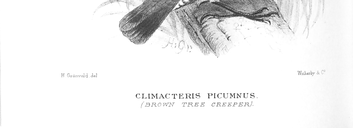
crop_bird(filenames[1])

scientific name of birds on a drawing

It does look cleaner now!

Text extraction

Now is the actual OCR step! The tesseract package provides bindings to the Tesseract OCR engine, free software currently sponsored by Google. It is a powerful engine, with a ton of parameters. Here again, tweaking a lot is warranted. Particularly useful reads are hocr vignette and this Wiki page of Tesseract about improving the quality of the output. The hocr package might be of interest for post-processing of OCR results.

Below, the only option changed from default is the page segmentation mode choosing 1 for “Automatic page segmentation with Orientation and script detection (OSD)”. When using Latin instead of English training data the results were not as good.

One can use either tesseract::ocr for a file path, url, or raw vector to image, or magick::image_ocr for a magick object which is quite handy in our pipeline.

The function below also filters results of the OCR using language detection. By only keeping text recognized as either Latin or English by one of the two language detection packages cld2 and cld3 that are interfaces to Google compact language detectors 2 and 3, one gets a first quality filter. If not doing that, the output would contain more unusable text.

get_names <- function(image){
  filename <- attr(image, "filename")
  ocr_options <- list(tessedit_pageseg_mode = 1)

  text <- magick::image_ocr(image, options = ocr_options)
  text <- stringr::str_split(text, "\n", simplify = TRUE)
  text <- stringr::str_remove_all(text, "[0-9]")
  text <- stringr::str_remove_all(text, "[:punct:]")
  text <- trimws(text)
  text <- stringr::str_remove_all(text, "~")
  text <- text[text != ""]
  text <- tolower(text)

  # remove one letter words
  # https://stackoverflow.com/questions/31203843/r-find-and-remove-all-one-to-two-letter-words
  text <- stringr::str_remove_all(text, " *\\b[[:alpha:]]{1,2}\\b *")
  text <- text[text != ""]

  # keep only the words that are recognized as either Latin
  # or English by cld2 or cld3
  if(length(text) > 0){
    results <- tibble::tibble(text = text,
                 cld2 = cld2::detect_language(text),
                 cld3 = cld3::detect_language(text),
                 filename = filename)

  results[results $cld2 %in% c("la", "en") |
          results$cld3 %in% c("la", "en"),]
  }else{
    return(NULL)
  }


}

(results1 <- filenames[1] %>%
  magick::image_read() %>%
  get_names())
## NULL

Nothing! Now if we replace magick::image_read with the previously defined crop_bird function that crops and cleans the image…

(results2 <- filenames[1] %>%
  crop_bird() %>%
  get_names())
## # A tibble: 2 x 4
##   text                 cld2  cld3  filename                          
##   <chr>                <chr> <chr> <chr>                             
## 1 climacteris picumnus <NA>  la    birds/n115_w1150_42399797481_o.jpg
## 2 brown tree creeper   en    <NA>  birds/n115_w1150_42399797481_o.jpg

We get a result! So we see that the image transformation was quite useful.

Now, these names look fine, but how to be sure they’re actually taxonomic names?

Taxonomic name resolution

The taxize package by Scott Chamberlain, is a taxonomic toolbelt for R, providing access to many fantastic data sources and tools for taxonomy. One of them, the Global Name Resolver, provides, well, resolution of taxonomic names, sadly not common names. taxize::gnr_resolve has many options, of which only one is used below: best_match_only = TRUE means it’ll only return the best match from the different data sources.

latin <- results2$text[results2$cld2 == "la"|
                         results2$cld3 == "la"]
taxize::gnr_resolve(latin,
  best_match_only = TRUE)
## # A tibble: 1 x 5
##   user_supplied_name submitted_name  matched_name   data_source_tit~ score
## * <chr>              <chr>           <chr>          <chr>            <dbl>
## 1 climacteris picum~ Climacteris pi~ Climacteris p~ NCBI             0.988

English names could be cleaned up a bit using the spelling package, also an rOpenSci package, since spelling::spell_check_text would output possible typos.

OCR bird naming workflow in action!

First the two steps image processing and OCR are applied to all images.

bird_names <- purrr::map(filenames, crop_bird) %>%
  purrr::map_df(get_names)

Out of 51 images only 17 are present in the final table with possible names which is a bit disheartening, but one could surely do better in the image processing and OCR tweaking steps! Maybe one could frame the parameter search as a machine learning problem. Please also keep in mind that such natural history images are quite hard to parse.

The name resolution information can be added to this table.

safe_resolve <- function(text){

  results <- taxize::gnr_resolve(text,
                                 best_match_only = TRUE)

  if(nrow(results) == 0){
    list(NULL)
  }else{
    list(results)
  }
}

bird_names <- dplyr::group_by(bird_names, text) %>%
  dplyr::mutate(gnr = ifelse(cld2 == "la" | cld3 == "la",
                             safe_resolve(text),
                             list(NULL)))

We do not get much resolution, but we knew the names weren’t very good to start with. A better (untested here!) idea here might be to get a full list of names of Australian birds, potentially leveraging the taxizedb package by Scott Chamberlain, and to then fuzzy-match them with the names we have.

unique(bird_names$gnr)
## [[1]]
## # A tibble: 1 x 5
##   user_supplied_name submitted_name  matched_name   data_source_tit~ score
## * <chr>              <chr>           <chr>          <chr>            <dbl>
## 1 climacteris picum~ Climacteris pi~ Climacteris p~ NCBI             0.988
## 
## [[2]]
## [1] NA
## 
## [[3]]
## NULL
## 
## [[4]]
## # A tibble: 1 x 5
##   user_supplied_na~ submitted_name  matched_name  data_source_title  score
## * <chr>             <chr>           <chr>         <chr>              <dbl>
## 1 austrodicaeum ii~ Austrodicaeum ~ Austrodicaeu~ The Interim Regis~  0.75
## 
## [[5]]
## # A tibble: 1 x 5
##   user_supplied_name submitted_name  matched_name   data_source_tit~ score
## * <chr>              <chr>           <chr>          <chr>            <dbl>
## 1 melithreptus laet~ Melithreptus l~ Melithreptus ~ CU*STAR          0.988
## 
## [[6]]
## # A tibble: 1 x 5
##   user_supplied_na~ submitted_name matched_name  data_source_title   score
## * <chr>             <chr>          <chr>         <chr>               <dbl>
## 1 rad isdlvorniode  Rad isdlvorni~ Rad Baker & ~ The Interim Regist~  0.75

Conclusion

rOpenSci packages supporting this (and your) workflow

In this post, we made use of R packages quite useful to wrangle information from diverse formats:

  • magick for image manipulation,
  • tesseract for optical character recognition (OCR),
  • cld2/cld3 for language detection.

We also used a function from taxize allowing us to use the Global Name Resolver. Discover more packages from our suite here.

Applicability of this OCR bird naming workflow

Actually, the BHL itself provides OCR output for its collection, see this example. I wasn’t able to find information about the software powering this OCR. What I was able to find out is that the BHL uses purposeful gaming in its OCR workflow. The raw OCR results aren’t much better than what we got in this post which is comforting.

More data from the Biodiversity Heritage Library

If you’re interested in other types of data from the BHL, in addition to the images, have a look at the rbhl package, part of rOpenSci’s suite, that interacts with the BHL API. One can e.g. search all books by the same author as the one we used images from.

author <- rbhl::bhl_authorsearch("Gregory M Mathews")
books <- rbhl::bhl_getauthortitles(creatorid = author$CreatorID)
head(books$FullTitle)
## [1] "A manual of the birds of Australia,"                                                                                                                                                                                                                                          
## [2] "A list of the birds of the Phillipian sub-region : which do not occur in Australia. "                                                                                                                                                                                         
## [3] "A manual of the birds of Australia /"                                                                                                                                                                                                                                         
## [4] "A list of the birds of Australia : containing the names and synonyms connected with each genus, species, and subspecies of birds found in Australia, at present known to the author /"                                                                                        
## [5] "Austral avian record; a scientific journal devoted primarily to the study of the Australian avifauna."                                                                                                                                                                        
## [6] "Arcana, or, The museum of natural history : containing the most recent discovered objects : embellished with coloured plates, and corresponding descriptions : with extracts relating to animals, and remarks of celebrated travellers; combining a general survey of nature."

Or we could get all books whose title contains the words “birds” and “australia”.

australia_birds <- rbhl::bhl_booksearch(title = "birds Australia")
head(australia_birds$FullTitle)
## [1] "Handbook to the birds of Australia. : [Supplementary material in Charles Darwin's copy]."
## [2] "An introduction to The birds of Australia /"                                             
## [3] "The useful birds of southern Australia : with notes on other birds /"                    
## [4] "The Birds of Australia"                                                                  
## [5] "The birds of Australia,"                                                                 
## [6] "The birds of Australia,"

And to get the OCR results of the pages of the book we used, we could write:

library("magrittr")

# ocr=TRUE to extract OCR for all pages
rbhl::bhl_getitempages("250938", ocr = TRUE) %>%
  # for each page transform the type into a string
  dplyr::group_by(PageUrl) %>%
  dplyr::mutate(page_type = toString(PageTypes[[1]])) %>%
  # keep only the illustration pages
  # that are like the ones we used 
  dplyr::filter(page_type == "Illustration") %>%
  # from the data.frame extract the OCR
  dplyr::pull(OcrText) %>%
  head()
## [1] "491 \nFAL CUNCULUS LEUCOGASTER. \n( WHITE -BELLIED £ If BIKE - TIT) \nFALCUNCULUS FRONTATUS. \nSHRIKE - TIT). \n"                                                                                                                   
## [2] "492 \nA** \nOREOICA GUTTURALIS. \n(CRESTED BELL-BIRD). \n"                                                                                                                                                                          
## [3] "APHELOCEPHALA LEUCOPSIS \n( WHITE FACE ). \n"                                                                                                                                                                                       
## [4] "* \nAPHELOCEPHALA PE CTORALIS. \n(CHE <3 TNUT -BREASTED WHITEFA CEj. \nAPHELOCEPHALA NIGRICINCTA. \n(BE A CK-BAH.DED WHITE FA CEj. \n"                                                                                              
## [5] "H . Gronvold. del. \nWitherLy & C° \nSPHENOSTOMA CRIS TATUM \n(WEDGE BIEL). \n"                                                                                                                                                     
## [6] "49 6 \nH \n(jronvolcl. del. \nN E O SIT TA LE CJ C O CE PHAI.A. \n( WHITE ¦ HE AID EE THE EH UN HE FL). \nNEOSHTA ALBATA \n(F IE E> T Ft E EE UNNEFlj. \nNEOSITTA CHRYSOPTERA \nf OFi. A. NGE - wing-e d tree runner). \nWitWLjA \n"

So there’s quite a lot to explore!

More birding soon!

Follow this series on the rOpenSci blog to explore this topic further! In the meantime, happy birding!

October 4, 2018by michelle.underhill

Help Support BHL

BHL's existence depends on the financial support of its patrons. Help us keep this free resource alive!

search

About BHL

The Biodiversity Heritage Library (BHL) is the world’s largest open access digital library for biodiversity literature and archives. BHL operates as a worldwide consortium of natural history, botanical, research, and national libraries working together to digitize the natural history literature held in their collections and make it freely available for open access as part of a global “biodiversity community.”

Join Our Mailing List

Sign up to receive the latest news, content highlights, and promotions.

Subscribe Now

Subscribe to Blog via Email

Enter your email address to subscribe to this blog and receive notifications of new posts by email.

Join 319 other subscribers

Subscribe to Blog Via RSS

Subscribe to the blog RSS feed to stay up-to-date on all the latest BHL posts.

Access RSS Feed

Inspiring Discovery through Free Access to Biodiversity Knowledge.

The Biodiversity Heritage Library makes it easier than ever for you to access the information you need to study and explore life on Earth…for free, anytime, anywhere.


64+ Million Pages of
Biodiversity Literature Online.

EXPLORE

Tools and Services
to Transform Research.

EXPLORE

300,000+
Illustrations on Flickr.

EXPLORE

ABOUT | HARMFUL CONTENT | PRIVACY | SITE MAP | TERMS OF USE